Practical introduction to Deep Learning using deeplearning4j

Deep What ?!

Let's start by exploring what does the deep in deep learning indicate?! As you probably know, the human brain is a circuit structure, and that structure is really complicated. It is made up of an intricate circuit piled up in many layers.

Hence, deep learning took the approach of making each layer learn in advance. This is literally known as pretraining. In pretraining, learning starts from the lower-dimension layer in order. Then, the data that is learned in the lower layer is treated as input data for the next layer. This way, machines become able to take a step by learning a feature of a low layer at the low-grade layer and gradually learning a feature of a higher grade. For example, when learning what a cat is, the first layer is an outline, the next layer is the shape of its eyes and nose, the next layer is a picture of a face, the next layers is the detail of a face, and so on. Similarly, it can be said that humans take the same learning steps as they catch the whole picture first and see the detailed features later. As each layer learns in stages, the feedback for an error of learning can also be done properly in each layer.

DeepLearning4j

A lot of the libraries of deep learning have been developed all over the world. When we look at the programming language with which libraries are being developed, most of them open to the public are developed by Python or use the Python API. TensorFlow is developed with C++ on the backend but it's also possible to write code with Python.

But wait, I'm a JVM fanboy! So, what JVM-based libraries do we have? Actually, there are a few cases that are actively developed (perhaps there are also some projects not open to public). However, there is only one library we can use practically: Deeplearning4j.

The the biggest feature of DL4J for me, is that it was designed on the premise of being integrated with Hadoop and spark. This indicates that DL4J suits the processing of large-scale data and is more scalable than other libraries. Moreover, DL4J supports GPU computing, so it's possible to process data even faster.

DL4J in practice

There are a plenty of examples of using DL4J that you can finf here. In this post, we'll build an image pipeline to prepare data for processing in a Neural Network using DeepLearning4. The source code for this simple example is available on github.

This repo contains, in addition to java main class, a testing and a training folder. each folder has 10 directories 0-9 in each directory are 28 * 28 grayscale pngs of handwritten digits. The training and testing directories contain 70,000 handwritten numbers data from 0 to 9, with both a height and width of 28 pixels each.

Main java class

The simple code contains only one class that handles everything.
First, we define the values necessary for the model:

    int height = 28; // The number of rows of a matrix.
    int width = 28; // The number of columns of a matrix.
    int channels = 1; // grayscale implies single channel
    int rngseed = 123; // This random-number generator applies a seed to ensure that the same initial weights are used when training. We’ll explain why this matters later.
    Random randNumGen = new Random(rngseed);
    int batchSize = 128; // How many examples to fetch with each step.
    int outputNum = 10; // Number of possible outcomes (e.g. labels 0 through 9).
    int numEpochs = 1; // An epoch is a complete pass through a given dataset.

Since images in our dataset are all grayscale data, the number of channels is set to 1. Furthermore, the example contains 10 possible outcomes (the labels numbered 0 - 9) which is our outputNum.

The next step is to get the path of our training and testing folders located on the ressources directory:

    File trainData = new File(ClassLoader.getSystemResource("training").getPath());
    File testData = new File(ClassLoader.getSystemResource("testing").getPath());

Now to process this data, we begin by defining a FileSplit

    FileSplit train = new FileSplit(trainData, NativeImageLoader.ALLOWED_FORMATS,randNumGen);
    FileSplit test = new FileSplit(testData,NativeImageLoader.ALLOWED_FORMATS,randNumGen);

Then we specify that we'll be reading the labels of images from the path:

    ParentPathLabelGenerator labelMaker = new ParentPathLabelGenerator();

    ImageRecordReader recordReader = new ImageRecordReader(height,width,channels,labelMaker);

After that we initialize the record reader and create one dataset DataSetIterator for training the model:

    recordReader.initialize(train);
    DataSetIterator dataIter = new RecordReaderDataSetIterator(recordReader,batchSize,1,outputNum);

Then, we set our hyperparameters (he quantities that define the architecture and how the algorithm learns.) and build the model layers (DenseLayer and OutputLayer).

    MultiLayerConfiguration conf = new NeuralNetConfiguration.Builder()
            .seed(rngseed)
            .optimizationAlgo(OptimizationAlgorithm.STOCHASTIC_GRADIENT_DESCENT)
            .iterations(1)
            .learningRate(0.006)
            .updater(Updater.NESTEROVS).momentum(0.9)
            .regularization(true).l2(1e-4)
            .list()
            .layer(0, new DenseLayer.Builder()
                    .nIn(height * width)
                    .nOut(100)
                    .activation(Activation.RELU)
                    .weightInit(WeightInit.XAVIER)
                    .build())
            .layer(1, new OutputLayer.Builder(LossFunctions.LossFunction.NEGATIVELOGLIKELIHOOD)
                    .nIn(100)
                    .nOut(outputNum)
                    .activation(Activation.SOFTMAX)
                    .weightInit(WeightInit.XAVIER)
                    .build())
            .pretrain(false).backprop(true)
            .setInputType(InputType.convolutional(height,width,channels))
            .build();

    MultiLayerNetwork model = new MultiLayerNetwork(conf);

After the building comes the training. Since we have multiple mini-batches, we need to iterate training through all the batches. Here, the test data and test labels are stocked for further use.

    for(int i = 0; i<numEpochs; i++){
        model.fit(dataIter);
    }

During the test, again, we need to iterate the evaluation process of the test data because we have more than one mini-batch:

    while(testIter.hasNext()){
        DataSet next = testIter.next();
        INDArray output = model.output(next.getFeatureMatrix());
        eval.eval(next.getLabels(),output);
    }

Then, we use the same as in the other examples:

    System.out.println(eval.stats());

This will return the result as follows:

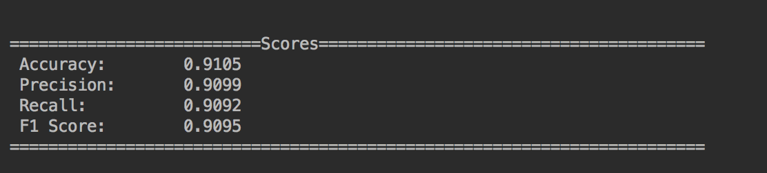
• Accuracy: The percentage of MNIST images that were correctly identified by our model.
• Precision: The number of true positives divided by the number of true positives and false positives.
• Recall: The number of true positives divided by the number of true positives and the number of false negatives.
• F1 Score: Weighted average of precision and recall.